10 Breakdown Systems

10   Breakdown Systems

1We start with the breakdown systems, because they provide some of the criteria for choosing a polyhedron. All systems start with a triangular polyhedron face and subdivide it with a three-way grid. We then push all the vertices of this grid outward till they are a common distance from the center (for spheres) or a harmoniously varying distance (for elliptical and other contours). When we have done this, some of the lines of subdivision will follow great circles inherent in the polyhedron’s symmetry. We want the ones that don’t do this to trace at least partial great circles, interrupted by the edges of polyhedron faces. And we want to maintain a reason- ably symmetrical spacing, so that the little triangles we have created will be nearly equilateral. We shall commence our thinking about all this by examining the first of the two basic ways to orient the grid.

10.1   Class I (Alternate)

2The grid lines run roughly parallel to the edges of the polyhedron face.

3 We want to specify the crossing points, and there are a number of different techniques, all of which yield slightly different strut lengths. All are correct, in the sense that they generate three-way grids with sphere vertices equidistant from the system center. Some are of historical interest chiefly. Still, there are choices to be made, and particularly at low frequencies we may be guided between two principal methods by a rather simple choice: similarity of triangle size, or similarity of triangle shape.

4 A worked example will clarify this. To keep figures few and simple we shall use the octahedron and compare two methods of making a $3v$ Class I breakdown.

5

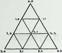
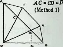
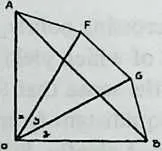
6 Diagrams 10.1 and 10.2 show Method 1. It amounts to drawing a triangle face on flat paper, dividing its edges equally, then projecting the division points outward to obtain equal radii. It is clear from Diagram 10.2 that although the divisions A C, CD, DB are equal, the chords AF, FG, GB are not (the end chords are shorter than the central one). The sighting angles from the center to the chord ends will differ likewise, so the $\mathrm{\Theta }$ coordinates will be unevenly spaced. Diagram 10.2 shows a construction for obtaining them. As for the triangle’s center point, we have learned that it is 54.7356° inward from each vertex (coordinates 45, 54.7356). Equation 9.2 will give us chord factors as shown.

31 Method 2¹ simply spaces the $\mathrm{\Theta }$ coordinates equally down th octa edge (30°, 60°, 90°), making all edge struts equal. The triangle’s center is located as before, and we proceed (Diagram 10.3) to obtain chord factors.

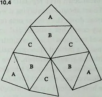
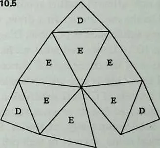
32 We should now look at models, and folding paper is an easy way to make them. Diagram 10.4 and Diagram 10.5 show patterns for one octa face computed by each method. Four of either, cut out and creased, can be taped together to make a hemispherical dome. By simply looking at the diagrams we can see a marked difference. When we have equal chord factors along the octa edge (Method 2), the small triangles vary less in size, but vary more in shape. Disregarding for the moment the comer triangles/1, which are always a special case, we notice that the rest of the octa face is shared by three each of two quite noticeably isosceles triangles, $B$ and C. But when we vary the edge chord factors (Method 1) the corner triangles $D$ stay virtually the same shape as before, while the rest of the octa face divides itself into 6 identical triangles $E$, which come much closer to being equilateral than either $B$ or Cin the other diagram.

33

34 In short, by letting the triangle sizes vary more we can keep their shapes more nearly constant.² This seems structurally as well as aesthetically preferable. The more nearly equilateral a triangle, the more nearly equilibrated should be its resistance to pushes and pulls from various directions. The price, a more marked variation in strut length, has been carried to extremes by the present example. It is less marked at high frequencies than at low, and less for the icosa than for the octa. A $3v$ octahedron is about the worst possible case.

35 0,0/1,0 0.517638

36 1,0/1,1 0.707107

37 2,0/2,1 0.650115

55method 2 coordinates

56 Since Method 1 appears to be the Class I breakdown of choice, we shall stick to it for the rest of the book.

57 A word about triangle shapes in general. Though the norm is an equilateral triangle, it is clear that if the little triangles were really equilateral we should have neither dome nor sphere but flat grid-work. It is their departure from equilaterality that provides the curvature, as we can see by considering the sum of the angles around a single vertex. Around the central vertex in Diagram 10.5, the apices of the $E$ triangles total 6 X 56.2°, or 337.2°. This is nearly 23° short of the 360° that would lie flat; the shortage is called the spherical excess of the vertex. Descartes showed long ago that the spherical excess of all the vertices in any polyhedron must always total 720°. Since there are 38 vertices in a $3v$ octa sphere, we should find an average spherical excess of nearly 19° at each of them. The vertex we have just looked at has more spherical excess than the average, and so have seven others like it; they are contributing to a deficit incurred at the vertices where four octa faces meet, and where 4 X 86.9° = 347.6° gives a spherical excess of barely more than 12°.

58 It is at these latter vertices—the octa’s six squares, the icosa’s twelve pentagons—that we are most likely to find deficient spherical excess, in other words a tendency to flatness. Flattish vertices are more likely to pop in under load, one reason it is desirable to keep spherical excess more or less evenly distributed (and triangles more or less equilateral).

59

10.2   Class II (Triacon)

60The grid lines run roughly perpendicular to the edges of the polyhedron face.

61

62 This breakdown has a reputation for being difficult to under- stand. To set about demystifying it we may note that it does not really break down the icosa or octa face from which it derives its frequency count, but a smaller and nonequilateral triangle which consists of two icosa or octa symmetry triangles back to back.

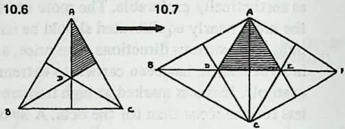
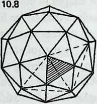
63 It arose as a method of incorporating the great circles that coincide with face-triangle medians. If we draw the three medians of a face we outline the symmetry triangles (Diagram 10.6). If we draw the medians of two adjacent icosa faces (Diagram 10.7) we find that we have outlined a pair of triangles, $\mathit{𝐴𝐷𝐸}$ and $\mathit{𝐷𝐸𝐶}$, each com- prising two symmetry triangles. If we continue in this way to sub- divide the entire icosa (Diagram 10.8) and then eliminate the icosa edges themselves, we have a $2v$ Class II breakdown, made up entirely of triangles like ADE.

64

65 If we now attempt further subdivision of the icosa face by lines parallel to the medians we first drew, we discover that only even-frequency subdivision is possible. Diagram 10.9 shows 4j>, and Diagram 10.10 shows that what we have really achieved is a $2v$ subdivision of the triangle ADE. Since in Diagram 10.8 we had covered the entire sphere with triangles like $\mathit{𝐴𝐷𝐸}$, such a triangle is the real module of Class II subdivision. There are sixty such triangles, clustered five to an icosa vertex, and they are what the Class II subdivision really subdivides. Since they seem to have no geometrical name, we may as well call them Class II triangles. (The diamond ADEC, made up of two of them, is one face of a spherical rhombic triacontahedron, hence the nickname triacon for this breakdown.)

66

67

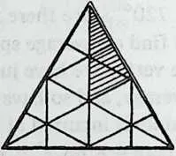
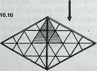
68 Once more there are several methods, of which we shall find uses for two.

69 Method 1 in effect divides the diamond median (= icosa or octa edge) exactly as in Class I, Method 1, to yield equal parts on flat paper but unequal chords when the vertices are pushed out to make spherical radii equal. We then concentrate on one half of the diamond, the Class II triangle, and run perpendiculars from the median outward to the sides. The triangle’s bottom edge is now subdivided the way its median was, and lines join these edgepoints to complete the grid.

70 The result is a strikingly symmetrical breakdown, and a little more economical of components than Class I, but not much. Its symmetry module is the icosa or octa symmetry triangle—that is, half a Class II triangle. (At first glance one might expect the module to be smaller, but the Class II triangle isn’t equilateral.)

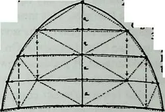
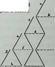
71 The other Class II system we shall find useful is called Method 3 in Clinton’s ‘‘Geodesic Math’’ article, where we find it credited to Duncan Stuart. It is one of the most ingenious achievements in the short history of geodesics, permitting as it does an absolute minimum member-length inventory - 4 for 4p, 12 for 1$2v$, and so on. We pay for its economy by accepting less symmetrical breakdown triangles. Diagram 10.11 shows the principle; the horizontal members cross the Class II triangle’s median at equally spaced intervals, and the bottom edge-point divisions are directly below the corres- ponding side-edge divisions (broken lines are at 90° angles with bottom edge). It now turns out (Diagram 10.12) that each side-edge division will propagate itself by zigzagging all the way down the main triangle, and each horizontal division will recur as a set of parallel reflections. The figure shows members of eight lengths for 8p. The chord factors show the asymmetries we accept; all members shorten as we move downward and outward.

72 Still, the saving in different member lengths is remarkable. This method requires 12 lengths for 12i>. A Class II Method 1 of the same frequency requires thirty-two, and a Class I Method 1 requires forty. It is not surprising that most of the largest geodesic structures hitherto have used Class II Method 3 components.

73 Of course we realize these savings only with spheres. Once the member length commences to vary with the radius, as in the case of ellipsoids, Method 3 loses all advantage over Method 1. For small Class II spheres, Method 1 gives visibly smoother arcs. But if you need to design a very large geodesic sphere and have any concern at all for economy of fabrication, Class II Method 3 is the place to start.

74l.a, a, a, a.

75 equal divisions of median.

76 2. Solid lines:

77

78Horizontals locate

79edge points.

80 3. Dashed lines:

81

82perpendiculars

83locate mid- and

84bottom points.

85 4. Dotted lines:

86 final grid.

87 10.11

88 METHOD 3 BREAKDOWN OF

89 CLASS II TRIANGLE, 8p.

90 10,12

91 SYMMETRIES

92 (LEFT HALF)

93 CHORD FACTORS

94$a$ 0.170287

95$b$ 0.199457

96$c$ 0.167003

97$d$ 0.195678

98$e$ 0.161026

99$f$ 0.184914

100$g$ 0.153316

101$h$ 0.168672

102 Values decrease

103 toward bottom

104 left (and, by

105 symmetry, toward

106 bottom right).

10.3   Which Class?

107We may now review the characteristics we have noted in passing.

108

109 Class I keeps component variations within narrower bounds, but does so at the cost of employing a larger inventory of different strut lengths (how much larger depends on the frequency, and increases rapidly). It permits odd as well as even frequencies, a greater advantage for simple systems than for complex. (Dropping from 4p to 3v permits notable economy; the saving of 1 Ip over 12p is quite unimportant.) Class I icosahedra have uninterrupted equators at all even frequencies, and at all frequencies numerous undulant lesser circles which we can straighten out by a method to be described later and use as truncation planes.

110 Class II yields even frequencies only. Used with the icosahedron (though not the octahedron or tetrahedron) it introduces some truncation problems, since any equator breaks through some of the subdividing triangles. This means figuring special members to close the gaps. The lengths of the several components vary over a wider range than Class I presents. On the other hand, Class II has economic advantages. It yields somewhat larger triangles for the same frequency than does Class I, somewhat fewer components, and somewhat fewer different components. In Method 3, as we have seen, the shrinkage of the list of different components can be spectacular. And we shall see in Chapter 16 its special advantages for diamond-pattern and space-frame applications.

10.4   Which Frequency?

111The smaller the polyhedron face we are subdividing, the lower the frequency we shall need for acceptable sphericity. And the larger the structure we intend to build, the higher the frequency we shall need, to keep component lengths reasonably short. High frequencies not only use a great many struts, they use a great many different strut lengths, a fact that is less apparent to the eye when the high frequency subdivides an icosa face than when we are dealing with an octa or, worse still, a tetra.

112 In general, to minimize component inventory, we use the lowest frequency we can. How long a component we can tolerate is a function of its slenderness ratio (length divided by diameter). Fuller has suggested 24/1 as a slenderness ratio for wood, 30/1 for metal or prestressed concrete.

113 Finally, very high frequencies bring each vertex so near to flatness as to be dangerous unless virtual thickness is imparted to the shell by trussing (see Chapter 16). ‘‘Very high,’’ for the icosa, means anything over 1$2v$ with careful workmanship, or over, say, $8v$ when tolerances are less than exacting.