12 Using the Tables

12   Using the Tables

1We now come to the actual coordinates and their use. Though a glance at the tables in Chapters 18--23 may suggest otherwise, the process by which they are obtained is almost ridiculously simple. Each $0,0$ pair is generated from a set of 3 integers whose sum is always the frequency of the breakdown, and for the octahedron, especially, the process of generation is so simple we seem closer to numerology than to engineering design. The following paragraphs explain how it is done for the reader who may some day want coordinates for some special frequency. The reader who simply wants to use the tables provided may skip to the next section of this chapter.

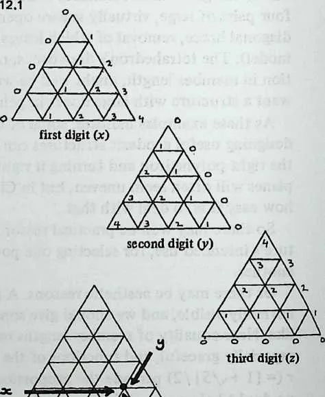
2 Diagram 12.1 shows how we get our sets of three integers. A diagram of one subdivided face is first numbered in the orderly fashion shown in the first drawing; this gives us the first integer of each vertex. The pattern is then rotated $60^{\circ }$ clockwise to obtain the second integer, and $60^{\circ }$ clockwise again to obtain the third.

3 Each vertex has now a unique three-integer label, and if we have made no mistakes, the sum of the integers at any vertex will always equal the frequency. Call these integers $x,y,z$.

4 Now for the octahedron,

5 For the icosahedron, we obtain $x,y,z$ in exactly the same way, but before using the equations we convert $x,y,z$ into $x_1,y_1,z_1$, as follows:

6

7 Here $\tau$ is the famous Golden Proportion, $(1+\sqrt{5})∕2$, or $1.61803399$, or $2\cos <!--\; FUNCTION\; APPLICATION\; -->36^{\circ }$ (this last form is the handiest to enter on the calculator). The icosa coordinates are:

8 For the tetrahedron, we convert $x,y,z$ into $x_2,y_2,z_2$, as follows:

9 The tetra coordinates are:

10 This system gives us Method 1 coordinates. For Class II Method 3 (inferior symmetry, but maximum component economy) we require another system, which is explained in Appendix 3.

11 Inspection of the octa and tetra equations discloses the useful fact that all coordinates for these polyhedra are either rational fractions or the roots of rational fractions. Thus $2,3,3$ in an $8v$ octa has the coordinates

12 Both values are given in the tables, but the former is quicker to enter on the calculator.

13 We shall now see how to use coordinates to design a geodesic structure.

12.1   Planning the Work: Class I

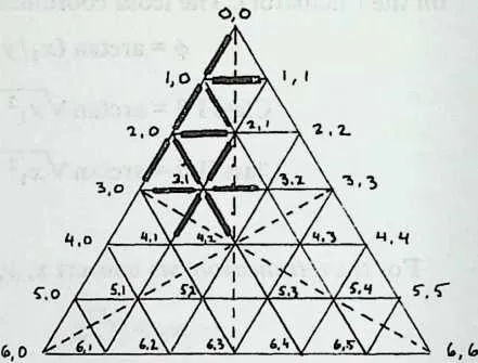
14Sketch an equilateral triangle (Diagram 12.2), subdivide the edges into $n$ parts for $n$ frequency, and join the points of subdivision with a three-way grid.

15 Now start with the top vertex $(0,0)$ and number all the crossing points, as shown. For frequency $n$ the last point on the bottom row will be $n,n$. Every point now has a two-digit marker.

16 Now draw the three medians of the face triangle (vertex to mid-point of opposite side: the broken lines in Diagram 12.2). You have outlined six right-angled triangles, each of which contains the whole symmetry system of the polyhedron. Concentrate on the top left one, which we’ll call ‘‘the’’ symmetry triangle. If the structure we are planning is spherical, we need chord factors only for the breakdown edges that lie partly or wholly inside the symmetry triangle. For the $6v$ example shown, this means only the twelve edges drawn with heavy lines: twelve out of sixty-three. For a sphere the only coordinates we need are the endpoints of those twelve edges: a total of ten coordinates. The rest of the system repeats symmetrically; thus $0,0∕1,0$ corresponds to $5,0∕6,0;6,0∕6,1;6,5∕6,6;5,5∕6,6;0,0∕1,1$: six occurrences of the one length. Anything that cuts an edge of the symmetry triangle occurs only three times per face: thus, $3,1∕3,2$ is repeated at $4,1∕5,2\mathit{𝑎𝑛𝑑}4,3∕5,3$.

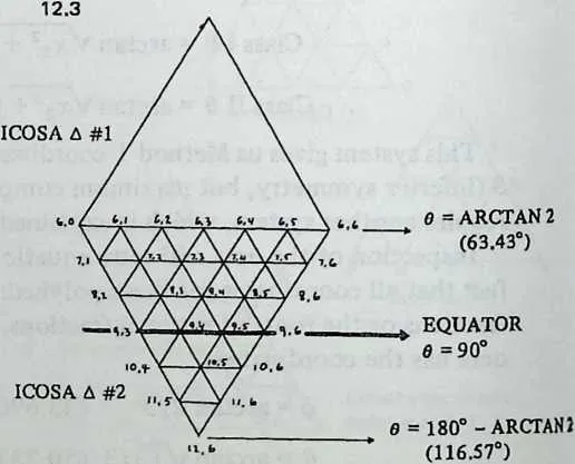
17 All this is true of spheres. If we plan something elliptical we need more lengths, because the radius changes constantly as we move down from the zenith $(0,0)$, and the top half of a face won’t duplicate the bottom half. We need coordinates as far down as $\mathrm{\Theta }=90^{\circ }$, where the bend of the elliptical contour reverses itself. An octa or tetra face goes down that far; an icosa face doesn’t, and the icosa tables provide for a second face, drawn under the first and numbered as shown in Diagram 12.3. (For more details see Chapter 13.) Because of the steadily altering radii the symmetry triangles no longer contain all the different lengths, but we still have left- and right-hand mirror symmetry to cut down our work.

18

19 We now make a list of the coordinates we actually require. To keep the example simple, we’ll stick to the sphere.

20 Each face has actually six symmetry triangles, and we’d get the same chord factors whichever we investigated. But we use the top left one because the numbers to be manipulated are handier if we stay to the left, where many $\varphi$ values are zero, and toward the top, where $0,0$ occurs and $\mathrm{\Theta }$ values are smallest. For a $6v$ sphere the worksheet would look like this:

50 Now we know which coordinates to extract from the table. Assume we want an icosahedral dome. We turn to ‘‘Icosahedron Class I Coordinates: Frequencies 6,3’’ (Chapter 20). Going down the ‘‘$6v$’’ column to the vertices we have just listed, we copy the coordinates as we find them. The list looks like this:

72 27.2237351

73 3,2 49.6138225

74 4,1 16.0353713

75 4,2 36

76 16.0353713

77 39.1034177

78 37.3773682

79 Now we are ready for chord factors. Since our structure is to be spherical we use Equation 9.2 and insert pairs of $\varphi ,\mathrm{\Theta }$ values from this table. Thus for the distance of $0,0∕1,1$ we use 0 for the values of ${\varphi }_1{\varphi }_2\mathit{𝑎𝑛𝑑}{\mathrm{\Theta }}_1$ and $9.3247035$ for ${\mathrm{\Theta }}_2$. The chord factor turns out to be $0.162567$. The reader should now practice with the calculator and the equation until he gets the following results. Once your routine is debugged you can work with great confidence.

80 We see that we have more symmetries than we had been led to expect: there are three identical pairs, hence only nine different component lengths overall. With experience such duplications can be anticipated. But it is always safer to invest a couple of minutes figuring a superfluous value or two than to waste time and building materials on a false assumption.

81 A way of checking the work is to list the coordinates inside a different symmetry triangle entirely and calculate the values for these. Though we are working with completely different numbers, the chord factors should be identical.

82 Note that the longest members radiate from the point $(4,2)$ where the symmetry triangles meet, and the shortest $(0,0∕1,0)$ from the comers of the face triangle. This is generally true of geodesic spheres, and gives us a quick test for improbable results. These two lengths are the extremes, and the rest should fall smoothly between them.

12.2   Accuracy

83We have given six-figure chord factors, and it is interesting to see what sort of accuracy this would yield in practice. We might envisage a hemispherical dome 100 feet in diameter (50-foot radius). This would entail strut lengths of the order of 10 feet, bigger than anyone is likely to go with 6v. The chord factor nearest the mean value $(0.196)$ is $0.198013$, and multiplying this by 50 feet we obtain a strut length for these particular members of 118.80780 inches. If we change the chord factor by +1 in the sixth place, we get 118.8084 inches, an error of 6 ten-thousandths of an inch. That is as much trouble as we are likely to get into by not using seven-place chord factors. Our coordinate tables are given to seven places (various rounding-off errors make the eighth place probable but not certain), so six places seems far enough to take chord factors.

12.3   Class II

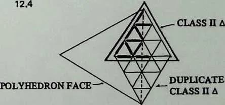
84The design of a Class II structure goes in the same way, with a few variations. The triangle we draw and subdivide is not the polyhedron face but its Class II triangle, as shown in Diagram 10.10. It straddles the edge between two polyhedron faces, and its bottom edge joins their centroids. For $n$-frequency division of the polyhedron, we make $n∕2$ subdivision of its Class II triangle, and our module of symmetry is the entire left-hand half of this triangle. Diagram 12.4 shows the idea. For a $6v$ Class II subdivision of the icosa face, we make a $3v$ subdivision of its Class II triangle. Chord factors for the left half of this are duplicated in the right half, and the entire Class II triangle is duplicated by mirror symetry below itself, bringing us to the end of an icosa edge, which we find we have thus divided into 6. So much for Class II spheres.

85

86 For the ellipse things are a little more complicated. To get down to the equator we need five symmetry triangles, as shown in Diagram 12.5 for an $8v$ example. Note carefully how the numbering is done; the sequence 0,0; 1,0; 2,0; and so on proceeds down the left-hand edge, and such sequences as 4,0; 4,1; 4,2 follow the upward-slanting lines.

87

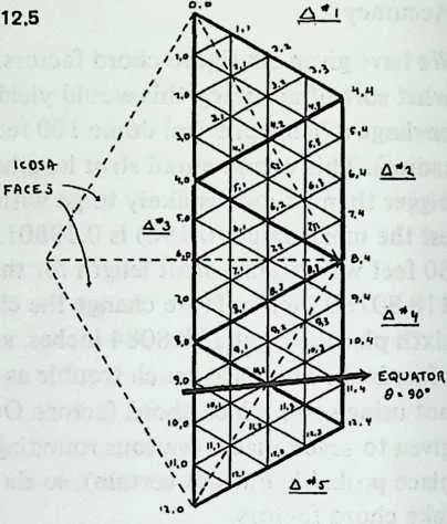
88 The equator $(\mathrm{\Theta }=90^{\circ })$ always passes through the midpoint of the edge the two bottom Class II triangles share (10,2 in the example) and passes a little below the edge point at the left, a little above the edge point at the right. A glance at the $8v$ icosa Class II Method 1 table confirms this; 1,0 has a 6 of 90, but the corresponding values for 9,0 and 11,4 are 88.95519820 and 91.04480176. So an equatorial cutoff just misses alternate vertices;

89 In Chapter 10 Class II Method 3 was presented as a system for maximizing the economy of different component lengths, at the cost of a slight loss in triangle regularity. Since this virtue applies only to spheres, the designer will be asking of this method none but spherical chord factors. So a complete set of these is provided in Chapter 23. They are ready for use without reference to the coordinates, which are presented only for their usefulness in two contingencies: the insertion of truncation planes (Chapter 14) and the design of space-frame structures (Chapter 16).

12.4   Appendix To Chapter 12: Derivation of the Coordinates

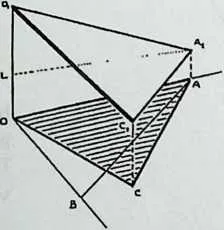
90Why the spherical coordinates are generated from triads of small integers we may learn from Diagram 12.6, which shows one face $\mathit{𝐴𝐵𝐶}$ of an octahedron with a $3v$ breakdown outlined upon it. The breakdown is projected downward onto the horizontal plane $\mathit{𝑂𝐵𝐶}$, every point on the projection lying directly beneath its original.

91

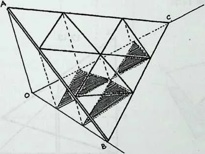
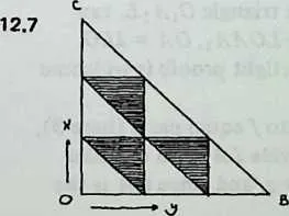
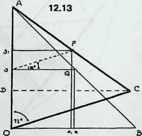
92 If we now look at the projection plane $\mathit{𝑂𝐵𝐶}$ by itself (Diagram 12.7) we see that it is a $45^{\circ }$ right-angled triangle, $\mathit{𝑂𝐵}$ and $\mathit{𝑂𝐶}$ indistinguishable from the Cartesian $x$ and $y$ axes. Thus all points on the projected breakdown have simple integral $x,y$ coordinates, and so do the points on the octa face directly above them ($p$ is at $1,1$).

93

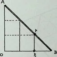
94 Diagram 12.8, a side view, shows how the $45^{\circ }$ slope of the octa face translates integral distances ($O-\mathit{𝑝𝑖}$) from the origin into integral verticals ($p_1-p$). Thus the $z$ coordinates of the breakdown vertices are also integral.

95

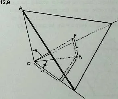
96 Turning now to Diagram 12.9, which is Diagram 12.6 redrawn with some details omitted, we see that the $\varphi$ of point $p$ is simply $\arctan <!--\; FUNCTION\; APPLICATION\; -->x∕y$. Its $\mathrm{\Theta }$ is $90^{\circ }-(\text{angle}\mathit{ 𝑝𝑂}{p}_1)$. Thus $\tan <!--\; FUNCTION\; APPLICATION\; -->\mathrm{\Theta }$ is $O{p}_1∕z$. Pythagoras tells us that $O{p}_1=\sqrt{x^2+y^2}$ hence $\mathrm{\Theta }=\arctan <!--\; FUNCTION\; APPLICATION\; -->\sqrt{x^2+y^2}∕z$.

97

98

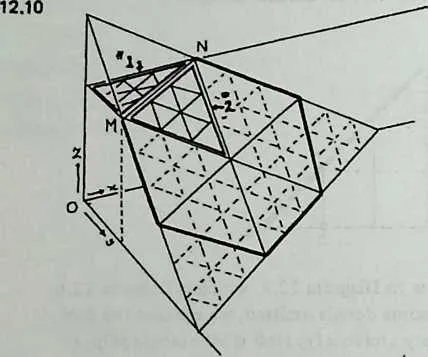
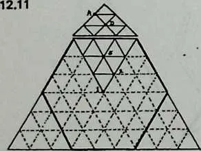
99 Before leaving the octahedron, we may recall A. J. Pugh’s observation that its truncated form, being a space-filling polyhedron, makes a sensible configuration to start from if we envisage clustered domes ((Polyhedra, University of California Press, 1976). The coordinates of truncated octahedral breakdowns are equally easy to write. Diagram 12.10shows why, to get a frequency $f$ (here $3v$) we start from an octahedral subdivision of 3/ (here 9p). We divide the octa face edges into thirds and fold the top corner back until it is parallel with the projection plane; it will become a quarter of the square face, our triangle 1. Its $x$ and $y$ values remain as they were, but its parallelism with the projection plane makes its z retain everywhere the value of z along line $\mathit{𝑀𝑁}$, that is, $2f$ (here = 6). Triangle 2 is a portion of the octa face, unchanged from its former orientation, so we can evaluate its points as if they were details in a 3/octa subdivision. Using our rule for writing the $x,y,z$ of single points, the reader can see that point 1 in Diagram 12.11 is at $3,3,3$; point 2 at $3,2,4$; point 4 at $2,2,5$; and so forth. And remembering to keep $z=2n$, he can identify point .4 as 0,1,6; point $D$ as $1,1,6$; and so on. Putting these values into the octahedron equations (Equation 12.1 and Equation 12.2) we can quickly derive the coordinates of all the points we need; thus $A$ is at $0,9.4623222$.

100

101 Diagram 12.12 shows what happens when we project an icosa face $O_1{A}_1{C}_1$ onto the plane where the Cartesian axes $\mathit{𝑂𝐵},\mathit{𝑂𝐴}$ are located. The $72^{\circ }$ angle at the icosa apex makes the projection lie skew. In Diagram 12.13 we see the projection $\mathit{𝐴𝑂𝐶}$ nestled between equal axes $\mathit{𝐴𝑂},\mathit{𝑂𝐵}$. The point $P$ is midway along $\mathit{𝐴𝐶}$; we choose this special case to keep the diagram simple, but any point on the icosa face would do. $\mathrm{\Theta }$ is similarly located at the midpoint of $\mathit{𝐴𝐵}$. Its coordinates are $x,y$, and we want to find the coordinates $x_1{y}_1$ of $P$. If $\mathit{𝑂𝐶}=\mathit{𝑂𝐵}=1$, it is easy to see that $\mathit{𝐷𝐶}=\sin <!--\; FUNCTION\; APPLICATION\; -->72^{\circ }$; $\mathit{𝐷𝐶}∕\mathit{𝑂𝐵}-\sin <!--\; FUNCTION\; APPLICATION\; -->72^{\circ }∕1$; and $x_1=x\sin <!--\; FUNCTION\; APPLICATION\; -->72^{\circ }$, as in Equation 12.4. Similarly, $y_1=y+\mathit{𝑃𝑄}$. But $\mathit{𝑃𝑄}∕x_1=\tan <!--\; FUNCTION\; APPLICATION\; -->18^{\circ }$, so $\mathit{𝑃𝑄}=(x\sin <!--\; FUNCTION\; APPLICATION\; -->72^{\circ })(\tan <!--\; FUNCTION\; APPLICATION\; -->18^{\circ })=x\cos <!--\; FUNCTION\; APPLICATION\; -->72^{\circ }$ Thus $y_1=y+x\cos <!--\; FUNCTION\; APPLICATION\; -->72^{\circ }$, as in Equation 12.5.

102 For $z_1$ we turn to Diagram 12.14, which is the rear wall of Diagram 12.12, with the same lettering. $O_1{A}_1$ is the icosa edge, $O_{1}O$ is the $z$ axis with $O$ at the center of the polyhedron. We shall take for granted two facts inherent in the icosa’s governing ratios: that in the triangle $O_1{A}_1{L}_1,\tan <!--\; FUNCTION\; APPLICATION\; -->A_1=1∕\tau$, and that in the rectangle $\mathit{𝐿𝑂𝐴}{A}_1,\mathit{𝑂𝐴}=2\mathit{𝐿𝑂}$. (The reader with an appetite for airtight proofs is welcome to construct them.)

103 We now divide the icosa edge into $f$ equal parts (here 3), and by dropping perpendiculars divide $L{A}_1$ and $\mathit{𝑂𝐴}$ likewise. We remember that $f=x+y+z$, and since $\mathit{𝑂𝐴}$ is the $y$-axis, $x=0$ and $z=f-y$ (again we are using a special case for simplicity). The $z_1$ into which we propose to convert this consists of two parts, the part in the triangle $O_1{A}_{1}L$, the part in the rectangle $\mathit{𝐿𝑂𝐴}{A}_1$. The former is $(f-y)∕\tan <!--\; FUNCTION\; APPLICATION\; -->A_1$, that is, $z∕\tau$. The latter is equivalent to $\mathit{𝐿𝑂}$, which is half $\mathit{𝑂𝐴}$; but $\mathit{𝑂𝐴}=f$. Hence $z_1=f∕2+z∕\tau$, as in Equation 12.6.

104 The tetrahedron is analyzed in the same manner, and the reader who wants proofs of Equation 12.10, Equation 12.11, and Equation 12.12 should have no difficulty working them out.

105