15 An Advanced Problem

15   An Advanced Problem

1Among the means at our disposal we may now list the following:

• Writing the 0,6 coordinates for Class I or Class II breakdowns of icosa, octa, or tetra polyhedra (Chapter 12, data in Part 3).
• Obtaining the distance (chord factor) between any two points on a spherical contour (Equation 9.2).
• Writing the third coordinate, r, for any 0 when the floor plan is circular and the silhouette is elliptical or superelliptical (Equations 13.1, 13.3, 13.4).
• Writing the third coordinate, r, for any 0,0 when both floor plan and silhouette are elliptical or superelliptical (Equation 13.7).
• Correcting for uneven expansion (Equations 13.2, 13.8, 13.9).
• Obtaining the distance (chord factor) between any two points on a nonspherical contour, once we have their three coordinates 0, 0, and $r$ (Equation 9.1).
• Inserting truncation planes at will (Chapter 14).
• Rotating the coordinate system to bring any point to the zenith (Equations 14.1,14.2).

2 We may now want to tackle a sophisticated problem that tests our resources. The harvest of insights seems to be worth the few pages we shall need to work it out in full. The reader who wants to test his command of the equations can spot-check any result at any point.

3 Near the end of Chapter 13 we were considering a superelliptical floor plan and contour, with a supercircular cross section. This offers the advantage of considerable floor space, with headroom maintained well out from the center. Because it is symmetrical by quadrants, it invites the use of the octahedron, one face triangle of which yields one quadrant exactly.

4 Unfortunately, it compounds a defect of the octahedron, deficient spherical excess at the principal vertices. If we are standing inside an octahedral geodesic hemisphere, a four-way vertex is directly overhead. If the breakdown is 4-frequency, the radials of this vertex will have chord factors of 0.141778, bounded by a square whose sides are 0.200000. These are almost right-angled triangles; the four angles meeting at the vertex are each 89.7121°, alarmingly close to the 90° which would make this vertex perfectly flat. Octahedral spheres are feasible because the small flat area is fully surrounded by vertices whose departure from flatness is correspondingly more emphatic. There is nothing wrong with flat vertices properly distributed. Fuller himself pioneered the hexpent configuration, which replaces pentagonal and hexagonal arrays with flat plates, in effect flattening numerous vertices throughout the system and relying on surrounding tensional grids to hold things together, and numerous hex-pent radomes have been withstanding Arctic winds on the DEW line for many years.

5 But once we introduce the superspherical or superelliptical contour, we find that quasiflatness is creeping a considerable distance out from the zenith. Not only is the zenith of the octa nearly flat, but so are the four vertices around it. Try the icosa- hedron. The angles around the pent vertex of a $4v$ sphere are each 71.3316°, so five total 356.658°. The four octa angles totaled 358.848°, so the icosa is helpfully less flat.

6 Now try it with the superellipse. We shall be using the same parameters throughout this chapter: floor expansion, 1.5; roofline expansion, 1,0; both exponents, 2.5. Above the superelliptical floor, we have a supercircle profile in one cross section, a super-ellipse profile in the other. So if the pent vertex overhead has a radius of 1, the 5 vertices surrounding it have radii greater than 1, pushing the ends of the radials out toward flatness. Calculating radii and chord factors, we find that the. 5 pent angles are each 71.985°, or 359.925° for the set—virtually flat.

7 Moreover, we have quadrant symmetry, and the icosa with its 72° radials will be awkward to quarter.

8 The solution, discovered by Bill Wild of Vail, Colorado, whose results appear without commentary in Shelter (Bolinas, Ca.: Shelter Publications, 1973) p. 126, is to move the icosa vertices away from the zenith. Move an edge to the zenith, and let it follow the super circular profile, so that the pent vertices at its ends will be carried down to where curvature is accentuated. Then instead of having less spherical excess than when the envelope is a sphere, they will have more. And overhead there will be no vertex at all to suffer that undue flatness (Diagram 15.1).

9 There is a bonus. With an edge up, the icosa will quarter neatly, the cuts running along that edge and straight down the centers of face triangles.

10 To achieve this we do the following:

1.

Discover how much of the icosahedron we shall need to account for, to include all points in a quadrant of a hemisphere.

2.

Write the coordinates of these points.

3.

Rotate the system of coordinates till the center of an icosa edge is at 0,0.

4.

Obtain the radii of all points in this new position.

5.

Obtain the chord factors.

6.

Attend to any truncation problems.

15.1   Quartering the Icosa

11Diagram 15.2 shows the situation. The icosahedron is edge-upward, and the fifteen great circles are marked on it. Their 90° intersections at face-triangle edges give us just the demarcations we want; as the diagram shows, a full icosa triangle plus halves of three others will exactly cover one quadrant of a hemisphere. (This makes 2 1/2 triangles, and since 4X21/2=10, our result agrees with the fact that 20/2 =10 icosa triangles would constitute a hemisphere.)

15.2   Writing the Coordinates

12Look at Diagram 15.3. The line 0,0-4,0 is the edge that will move to zenith. The full triangle we want is the second icosa triangle in the tables, 4,0-4,4-8,4. Of the upper icosa triangle (0,0-4,0-4,4) we need only half, as shown. Since two struts pass across its upper boundary, we also need points 2,1 and 3,3. All these points are obtained directly from the tables.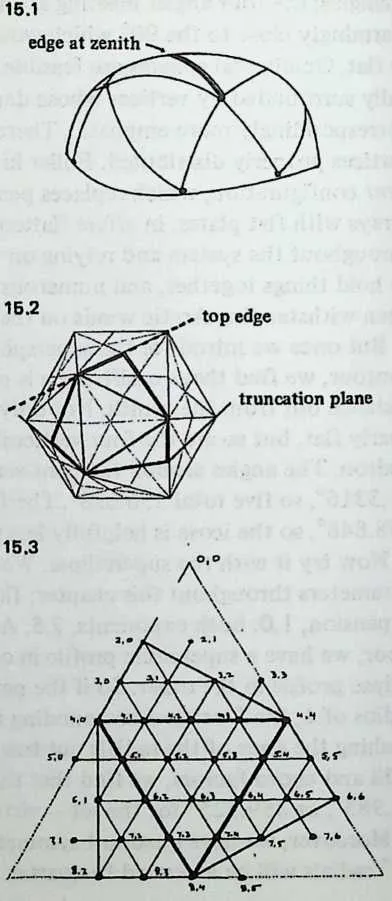

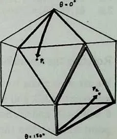
13 To obtain coordinates for the part-triangles 4,0-8,2-8,4 and 4,4-8,4-6,6 we remember how the icosa is put together (see Diagram 15.4). These are also second triangles, but up-pointing. Any point in them will be the same distance from the bottom icosa vertex (0 = 180°) as the corresponding point in the usual second triangle is from the top vertex (6 = 0°). So we identify corresponding points and subtract from 180°. Thus 7,2 corresponds to 5,2; subtracting the 0 of 5,2 from 180°, we obtain a 0 for 7,2: 106.0450570°.

14 To obtain the 0 values of these points, we note that symmetry places them left and right of icosa-triangle centerlines exactly as the corresponding points in the second triangle are placed left and right of its centerline. Its centerline is at 0 = 36°. The up-pointing triangle centerlines are at 0 = 0° and 0 = 72°. Since 5,2 is 36° - 26.2676986° = 9.7323014° from the 36° centerline, the 0 of 7,2 is 0 + 9.732014 = 9.7323014°, and the 0 of 7,5 is 72 - 9.7323014 = 62.2676986°.

15 Again notice that edge-crossing struts will require us to write some coordinates outside these boundaries. Since 5,0 and 7,1 are to the left of the 0 = 0 line, their 0 values are negative. Table 15.1 lists all of the coordinates we require.

16

17TABLE 15.1 Coordinates from Table

15.3   Rotating the Coordinate System

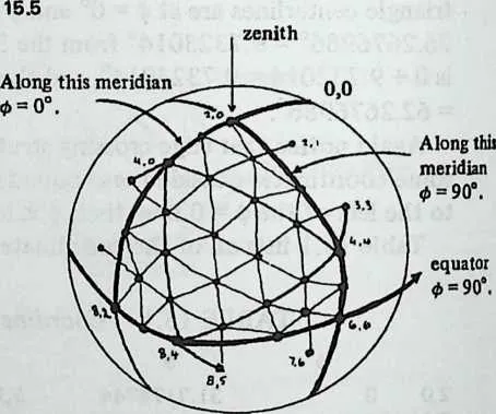
126We are now going to move the midpoint of the edge 0,0-4,0. This midpoint is 2,0, and since it will now occupy the zenith, its 0 and 0 will be 0° and 0°. So we want to know what the 0 and 9 of each point will be when the present 0, 31.71747438 has been moved to 0,0. Equation 18.1 and Equation 18.2 give us the answers, with tedium but not difficulty. One caution is needed: we must watch that we assign 0 to the right quadrant. Diagram 15.5 shows the new boundaries: normally all values will lie between 0 and 90. Thus 8,5 and 7,6 are the only points below the equator. Here Equation 14.1 will give us the proper 9 values. Point 2,1, however, lies beyond 0 = 90°, and here we confront the fact that Equation 14.2 yields its answer as an arcsine, in this case arcsine 0.8506508. The unthinking answer is 58.2825260. But we need something greater than 90°; the value we want must be in the second quadrant, 121.7174740. Similarly, the 0 values for 5,0 and 7,1 must be negative but not a great deal less than zero: they are in fact the negative values of their counterparts 5,1 and 7,2. An eye kept on the diagram’s physical realities will prevent mistakes.

127 Table 15.2 shows the rotated coordinates. To prevent confusion the points keep their old labels.

128

272 If we intend to alter the coordinate symmetry with the help of Equations 13.8 and 13.9, now is the time to do it. To shorten the example we’ll skip this option, remarking only that since the floor is being expanded along the 0 = 90° axis, both equations would require the modification explained previously.

15.4   Tabulating the Radii

273Again the work is tedious but perfectly straightforward. There is only one thing to remember: the direction of the long axis of the floor. With a vertex at the zenith—the usual situation—this is unimportant, but here we want to be sure that the vertexial edge runs along the supercircular rooftree, not the superelliptical one. This is chiefly to work the pent centers at the ends of this icosa edge as far down into the zone of curvature as we can. (It also happens to yield a tighter clustering of chord factors.) Now Equation 13.5 as it stands will expand the floor along the $\varphi =0$ axis, which is 90° from where we want it. The easiest way to swing things 90° is to alter Equation 13.7 very slightly; we have only to interchange $\sin <!--\; FUNCTION\; APPLICATION\; -->\varphi$ and $\cos <!--\; FUNCTION\; APPLICATION\; -->\varphi$, and Equation 13.7 will swing the floor plan as we want, and generate the radii as tabulated in the right-hand column of Table 15.2.

15.5   Chord Factors

274This is the ungrateful case where symmetry fails us on any scale smaller than 1 /8 sphere; hence, we need chord factors for all the struts in the dome quadrant. A good way not to miss any is to mark each strut red on a diagram as its value is computed.

275 Equation 9.1 will give the values in Table 15.3. They do not correspond to those shown by Mr. Wild in Shelter because his expansion was only 1.25, while ours is 1.5. A model will tell us whether we like the looks of it; if not, we can go back to Mr. Wild’s stubbier form. (Refigure radii, refigure chord factors.)

276

277TABLE 15.3 Chord Factors

368

369TABLE 15.3 Chord Factors (continued)

15.6   Truncation

424Just a small problem. Though we are using an even-frequency icosahedron, the rotation to edge zenith has a great-circle equator that cuts through triangles. This is the same great circle that supplies broken equators for Class II breakdowns, and it is dealt with in the same way: we figure special members to close the gaps where they occur.

425 It turns out that we don’t want 7,4/8,5 and 6,5/7,6 after all, unless to construct a sphere model. We want midpoints, 8,5 and 7,6 (italicized to denote a change) between points 8,4-7,5 and 7,5-6,6, and we want a total of 6 new members to join things up. The new coordinates are:

426

4278,5 45.0000000 90 1.2494849

4287,6 74.1412628 90 1.4910254

429 The $\varphi$ values simply split the difference between the ones on either side of them. The 6 values are manifestly 90°. The radii are obtained as usual. The chord factors for the truncation members are then:

430 7,4/<?,5

431 8,4/<8,5

43275/8,5

433 0.187102

434 0.300297

435 0.333335

436 6,5/ 7,6

437 7,5/7,6

4386,617,6

439 0.243588

440 0.410359

441 0.412714

442 The complete dome will require four members of each of these lengths.

443 This completes the work. Which angles, if any, we may need to calculate will depend on the envisaged method of construction. How to do this, and how much of it to do, are outlined in Chapter 17.