9 The Spherical-Coordinate System

1We have learned that two angles—call them $ϕ$ and $Θ$ will specify a direction, and two angles $ϕ, Θ$ , together with a distance $r$ will specify a unique point. These are the elements of the spherical- coordinate system, which is less well known than it might be. Most problems of geodesic mathematics can be solved with its aid with straightforward ease.

2 The $ϕ$ coordinate resembles a meridian of longitude. All points with the same $ϕ$ lie on the same great circle, which passes through the zenith $(0, 0)$ . It is convenient to incorporate the reference meridian, $ϕ = 0$ , into our calculations whenever we can. The first coordinate of all points situated on it will be 0. The $Θ$ coordinate resembles a specification of latitude, except that it is measured down the $ϕ$ circle from $0^{\circ}$ at the zenith, instead of upward from the equator. (In the spherical-coordinate system, the equator is at $Θ = 9 0^{\circ}$ .) All points whose second coordinate $Θ$ is $90$ lie on the equatorial great circle. With the exception of these, all points with the same $Θ$ lie on the same lesser circle and specify a plane along which the dome can be truncated so it will sit flat.

3 The $r$ coordinate, measured not in degrees but in units of length from the center, tells us how far out a point is to be found. If the points are on the surface of a sphere, like the vertices of a spherical geodesic structure, we can let $r = 1$ and virtually disregard it. The angles $ϕ$ and $Θ$ tell us all we need to know. If the envelope of the system is other than spherical, then varying values of $r$ will have to be taken into account.

4 Now for the usefulness of understanding this system. If we know the coordinates $ϕ_{1}, Θ_{1}, r_{1}$ and $ϕ_{2}, Θ_{2}, r_{2}$ of two points, then we can find the distance between them by inserting these values into an equation which a pocket calculator can readily subdue. The result, $d$ , will be in the unit used for $r_{1}$ and $r_{2}$ , and if either of these distances—or both in the case of a sphere—is made equal to 1, the result will be a chord factor.

d = \sqrt{r_{1}^{2} + r_{2}^{2} - 2 r_{1} r_{2} {\cos Θ_{1} \cos Θ_{2} + \cos (ϕ_{1} - ϕ_{2}) \sin Θ_{1} \sin Θ_{2}}} .

(9.1)

5 For the spherical case, when $r_{1} = r_{2} = 1$ , this becomes

d = \sqrt{2 - 2 {\cos Θ_{1} \cos Θ_{2} + \cos (ϕ_{1} - ϕ_{2}) \sin Θ_{1} \sin Θ_{2}}} .

(9.2)

6 For a first example, check back to the $2 v$ octahedron we discussed in Chapter 5 (Diagram 5.4). Diagram 9.1, with the same lettering, shows how this looks in spherical coordinates. $A, B, C$ , are the corners of one octahedral face. Their $0, 0$ coordinates are $0, 0; 0, 90; 90, 90$ . The edge midpoints $M_{1}, M_{2}, M_{3}$ have the coordinates $0, 45; 90, 45; 45, 90$ . Because the system is symmetrical we need only two distances: a vertex to a midpoint, and a midpoint to a midpoint. $A - M_{1}$ and $M - M_{2}$ will suffice. Because the system is spherical we use Equation 9.2. The sines and cosines we shall need are as follows:

	cosine	sine
$0^{\circ}$	0	1
$4 5^{\circ}$	0.70710678	0.70710678
$9 0^{\circ}$	1	0

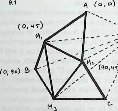
8 Inserting these values into Equation 9.2, we get for $A - M_{1}$ (coordinates $0, 0$ and $0, 45$ ):

9 d=V2- 2(0.70710678 + 0)

10
11=V2 - 1.41421356 =V0.58578644 = 0.765367

12 And for $M_{2} - M_{2}$ (coordinates 0,45 and-90,45) we get

13
14d=V2- 2(0.5 + 0)
15= V1
16= 1.0

17 These answers agree exactly with those we obtained by other means in Chapters 5 (Diagram 5.5). And since they are multiples of $r$ when $r = 1$ , they are identical with the chord factors introduced in Chapter 8.

18 True, the purely geometrical argument in Chapter 5 yielded the chord factors with less manipulation and in less time. But that was a $2 v$ case. Raise the frequency, and the geometrical method soon becomes too cumbersome to stay in the running. (Desert the spherical contour, and it becomes nearly impossible.) Moreover, each result yields data for its successor, and an early error invalidates subsequent work. The 0,0 method, on the other hand, permits a standardized procedure. All chord factors are found by exactly the same routine, and all are found independently; errors are isolated, and do not affect other computations. And a good pocket calculator, which can quickly change angles into their sines and cosines and has no more trouble with roots than with 2 4-2, permits us to run through the chord-factor equation for each pair of points in less than a minute, even when coordinates are cumbersome. (Suitably programmed, the ultra-sophisticated HP-65 will do the computing in four seconds per case.)

19 While we have in front of us data for a simple case, we may as well experiment with Equation 9.1. What if we wanted to make this simple dome elliptical? Let us specify a beehive orientation (Diagram 9.2) 11/2 times as high as it is wide. A hemisphere of 20-foot diameter would thus be stretched to give not 10 feet of headroom but 15.

20 We see at once that the radius varies with $d$ . At the zenith $(0 = 0)$ , $r = 1.5$ . At the floorline (0 = 90°), $r = 1.0$ . At the octa mid-edge (0 = 45°), the reader may take it on trust that $r = 1.1767$ . (We shall learn later how to calculate $r$ for any value of 0 in ellipses of any proportions.) These are the only values of 0 we have to deal with, so we make a $0 : r$ table:

21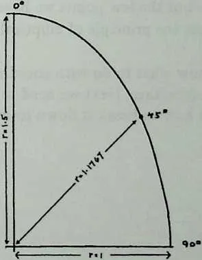 9.2

22e r

23 0° 1.5

24 45° 1.1767

25 90° 1.0

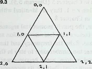
27 Since $r$ continues to vary beyond the confines of the octa symmetry triangle, we should identify the various vertices in a face triangle (Diagram 9.3 shows a useful notation) and decide how many different chord lengths we must deal with. 20/21 and 21/22, where $r = 1$ , will be just the same as before. But since 0,0 and 1,0 have special values for r, we shall need 10/11,00/10, 10/20, and 10/21. But the system retains mirror symmetry (1,0 has the same 0 as 1,1), so 00/11 will equal 00/10, 10/20 will equal 11/22, and 11/21 will equal 10/21. So we need four new chord factors, which we obtain by putting the proper values of 0, 9, and $r$ into Equation 9.1. Thus 10/21 is given by:

\begin{matrix} d = \sqrt{1.176 7^{2} + 1^{2} - 2 \times 1.1767 \times 1 (0.70710678 \times 0.70710678)} \\ = \sqrt{1.2079} \\ = 1.099 . \end{matrix}

28 The reader may verify that $00 ∕ 10$ is $1.067$ , $10 ∕ 20$ is $0.8488$ , and $10 ∕ 11$ is $1.1767$ .

29 A model built to these specifications would be far from smooth—the frequency is simply too low to record nuances of elliptical curvature—but the few points we have are correctly located, and it is clear that the principle of elliptical domes presents no real difficulties.

30 So we know what to do with coordinates of breakdown vertices on a polyhedron face. Next we need to know which polyhedron to choose, and how to break it down to obtain the coordinates themselves.